How I’m using Machine Learning to Trade in the Stock Market!

Disclaimer: This article is about a basic technique that I have used to make an exchanging bot. While back-testing shows that the exchanging bot is beneficial, the exchanging bot isn't fit for taking care of "dark swan" occasions, for example, market slumps. Additionally I am not a monetary consultant nor an expert broker. I'm essentially sharing this for amusement purposes. So exchange and read despite all advice to the contrary.

Back in my senior year of school I was first acquainted with the financial exchange by a companion. I purchased a stock that was suggested by a youtuber (not the most brilliant thing) and making a 100 percent return very quickly. This exchange was essential to the point that I actually recall the stock. The ticker image was AETI. Obviously it was novices karma, since I had no clue about the thing I was doing. From that point forward I have contributed a ton of time and cash into monetary business sectors and had a decent amount of gains and misfortunes. In spite of the fact that, I have been tolerably fruitful, I as of late found that I might have been more effective notwithstanding my feelings.

Since this disclosure, I have been searching for ways of moderating my feelings during contributing and exchanging. I understood the most ideal way to dispose of feelings is by making an exchanging bot. In the wake of investigating a few algorithmic exchanging systems, I chose to concoct my own model by using a fundamental AI model, Logistic Regression (LR).

Making the system..

The most major procedure in the securities exchange is purchasing low and selling high. Presently, assuming you have contributed or exchanged for quite a while, you'd know that it's not generally so natural as it sounds. Thus, I needed to make a model that predicts low's and high's of stocks as precisely as could be expected.

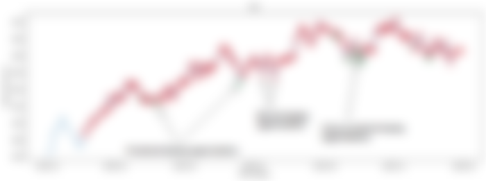
In Figure 1, you see Apple's day to day stock cost activity from year 2018 to 2021. The green dabs are nearby least qualities and red dabs are neighborhood greatest qualities. So my goal was to utilize ML and anticipate assuming an information point is a green speck (class 0) or a red dab (classification 1). The objective is to just purchase assuming that the model predicts a green point and sell when the stock cost goes up a specific rate.

Here are the four stages of my methodology

- Utilize the ML model to anticipate on the off chance that purchasing the stock is great on a specific day.

- If favorable(green specks) purchase the stock.

- When the stock ascents a specific rate sell the stock for an addition.

- Assuming the stock plunges a specific rate sell the stock for a misfortune.

Another subtleties

- The calculation will just hold each stock in turn (This was done to keep everything straightforward)

- The selling rates are two hyperparameters of the model that we can decide to amplify gains.

- On the off chance that you are pondering, "imagine a scenario in which the information point is neither a neighborhood max nor a nearby min?", hold tight we'll discuss this later on.

The ML model

As referenced over, the AI model I utilized was Logistic Regression (LR). In the event that you are curious about LR, you can actually look at my instructional exercise journal by clicking here.

In the first place, our concern is a twofold arrangement issue with two designated yields. In particular, neighborhood essentials (classification 0, 'green spots') and nearby maximums (classification 1, 'red specks'). Next we need to decide the contributions of the model. An extremely straightforward thought is to utilize the stock cost and the volume as contributions to the LR model and anticipate assuming it is a nearby least or a neighborhood greatest. Be that as it may, the stock cost and volume are almost no data to anticipate something as muddled as the heading of a stock. In this way, I furthermore elaborate four other information boundaries in my model.

Standardized stock cost - Instead of utilizing the stock value, I involved a standardized stock cost as my first info boundary. A stock's value activity can for the most part be portrayed by a candle as in Figure 2. The candle addresses the most elevated stock cost (HIGH), the least stock cost (LOW), the open stock cost (OPEN) and the nearby cost (CLOSE) for the afternoon (assuming we consider an everyday outline as in Figure 1). To make it more straightforward I made a solitary worth somewhere in the range of 0 and 1 addressing every one of the four of these qualities. This worth was determined by the Equation 1. Assuming the subsequent worth is near 1, this implies that the stock has shut close to the HIGH of the day, while on the off chance that the standardized worth is almost 0 it implies that the stock has shut close to the LOW of the day. The benefit of utilizing such a worth is that it contains data of the value activity of the entire day contrasted with utilizing a solitary worth like the CLOSE or the normal of the day. Additionally this worth isn't touchy to stock parts.

• Volume — The second parameter used in the model was the daily volume of the stock. This parameter represents the amount of shares traded (both bought and sold) on a specific day.

• 3 day regression coefficient — The next parameter was the 3 day regression coefficient. This was calculated by performing linear regression to the past three day closing prices. This represents the direction of the stock in the past three days.

• 5 day regression coefficient — A similar parameter to the 3 day regression coefficient. Instead of three days here I used five days.

• 10 day regression coefficient — Same as above, but used 10 day regression. This value represents the direction of the stock price in the past ten days.

• 20 day regression coefficient — Same as above, but used a 20 day regression.

Preparing and approving the model

In the wake of characterizing my model, I utilized the TD Ameritrade API to gather the verifiable information to prepare the model. The stocks used to make the dataset were the thirty organizations of the DOW 30 and twenty other noticeable organizations of the S&P 500. The preparation and approval information spread over between 2007 to 2020 (counting). The testing information was from 2021.

To set up the preparation and approval information, I previously observed information focuses addressing either a purchasing point (classification 0 or green dabs in Figure 1) or a selling point (classification 1). This was finished by a calculation made to look for nearby mins and max focuses. In the wake of choosing the elements, the volume information was gathered and the standardized cost esteem and relapse boundaries were determined. Figure 3 shows an example of information.

After preparing data, I used the scikit-learn package to split the data into train & validation sets and train the LR model. The LR model used the input parameters and predicted the target value.

Validation results and analysis

The validation set contained 507 data samples. The fully trained LR model was able to predict the validation data with a 88.5% accuracy.

This accuracy of the model at first seems to be very convincing. So let’s see how the model performs on a stock in year 2021. To do this I chose data from Goldman Sachs (stock ticker GS) and predicted the direction of the stock on each day using the trained LR model. The results are depicted in Figure 4.

Whenever you take a gander at Figure 4, you see that the model is anticipating a ton of misleading up-sides (up-sides being purchasing focuses). Despite the fact that it appears to foresee practically every one of the nearby essentials accurately, it erroneously anticipate purchasing focuses. On the off chance that you recall from the preparation stage, I just utilized nearby maximums and neighborhood essentials to prepare the model. So the model expectations on the moderate information focuses are exceptionally powerless.

This can be an expensive mix-up in contributing. All things considered, purchasing high and selling low isn't our goal 😬. Thus, how might we settle this and pick the purchasing focuses with more sureness. We should return to the approval results and check whether we can figure out how to expand the conviction of our purchasing focuses.

In Figure 5, you can see the disarray framework of the approval results. There are 29 examples that our model anticipated in class 0 (purchasing point/nearby least) when it was really a classification 1 (selling point/neighborhood greatest). These are bogus positive qualities (erroneously recognize negatives as up-sides. Additionally recall that for our situation up-sides are purchasing focuses). Assuming we review the methodology, the objective of my model was to observe purchasing focuses utilizing the ML model. So we can attempt to diminish these misleading up-sides and ensure the model predicts purchasing focuses with high sureness. We can do this by changing the edge of our LR model.

In Logistic Regression twofold order, the default edge is 0.5. Intending that assuming the modular predicts a likelihood more prominent than 0.5, that information test will fall into class 1 though in the event that the model predicts a likelihood under 0.5 the information point will fall in to classification 0. We can change this limit to build the certainty of the model forecasts of a specific class. For instance on the off chance that we change this edge to 0.1 just the forecasts under 0.1 will be chosen as purchasing focuses (class 0). This diminishes the quantity of misleading purchasing focuses as the model just chooses the examples that are close to 0.

So to ensure my model predicts purchasing focuses with more conviction. I changed the edge of my model to 0.03. (Note that this is only a model. We can later attempt to change the limit to tune the model to perform well). You can now see the new disarray framework in Figure 6.

As you can see now the number of false positives are zero. However, the downside of this is that the model misses a lot of true positive values. In our case the model only recognizes five buying points and misses to identify a lot of other buying points.

Now let’s use the new threshold and re-plot the buying points for the Goldman Sachs stock in 2021.

As you can find in Figure 7, presently the model predicts purchasing open doors with more sureness. Nonetheless, it additionally has botched a few purchasing open doors. This is the penance we need to make to purchase with high sureness.

Back-testing and results

Then, I back-tried my technique on 2021 financial exchange information. I made a stock test system and a back-testing script that outputs for purchasing valuable open doors in the DOW 30 regular utilizing the LR model and a given threshold(t). On the off chance that there is a stock accessible, the test system purchases the stock and holds the stock until it arrives at a specific rate gain(g), a specific rate loss(l) or a sells after a specific measure of days(d). The last back-testing recreations had four boundaries (t, g, l, d) and the objective was to augment benefit.

I likewise made four financial backer sorts by changing these boundaries. The "Restless Trader", "Moderate Holder", "Patient Swing Trader" and "The APE".

The Impatient Trader - This kind of broker purchases and holds the stock for an exceptionally brief timeframe. The broker likewise searches for little gains. This dealer is likewise frightened of misfortunes, so the merchant will in general sell the stock for a misfortune assuming that the stock drops even a tad. At last this merchant picks stocks with a high limit to rapidly find one more stock once they dispose of their present stock. Along these lines, boundaries for this kind of dealer are t = 0.3, g = 0.005, l = 0.001 and d = 3.

The Moderate Holder - This kind of dealer purchases and holds the stock for a moderate timeframe. The merchant is searching for stocks with high certainty so the edge esteem will in general be low. The merchant likewise searches for higher gains and has a higher capacity to bear misfortunes contrasted with the Impatient Trader. For this kind of dealer the boundaries are t = 0.1, g = 0.03, l = 0.03 and d = 10.

The Patient Swing Trader - As "swing" recommends, this kind of broker will in general hold the stock longer. Additionally the merchant likes to choose stocks with high likelihood of progress. So the limit is extremely low for this kind of broker. Additionally this broker trusts in selling stocks for more modest misfortunes and continuing on to various stocks. The boundaries for this kind of merchant are t = 0.05, g = 0.04, l = 0.003 and d = 21.

The APE - The APE is the kind of merchants that are new to the securities exchange. They will quite often pick stocks nonsensically. So the utilization no methodology to choose stocks. These kinds of financial backers haphazardly pick stocks and arbitrarily sell them at whatever point they feel like it.

Presently how about we run back-testing and perceive how the four financial backers perform. These reproductions depend on 2021 information and every financial backer is given a 3000 USD as their beginning equilibrium. The exhibition of every financial backer sort is measured toward the finish of 2021.

Figure 8, shows the results of how the four investors have performed. The “Patient Swing Trader” has been able to make the largest profit by making a 47.77% gain at the end of year 2021 followed by the impatient trader with a gain of 30.41%. As expected, the irrational trader “The APE” has the lowest returns with a 13.72% gain.

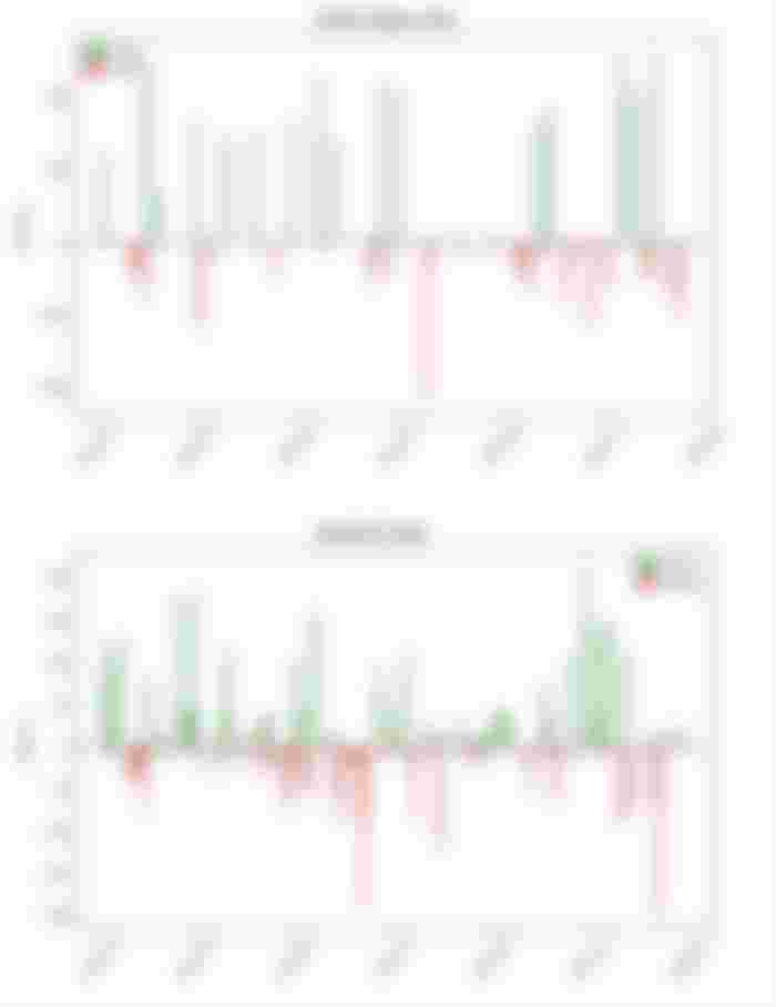
Figure 9 shows the win/loss bar plots for the “Patient Swing Trader” and the “Impatient Trader”. As expected, the patient swing trader has taken a small amount of trades and has cut losses as quickly as possible. The impatient trader has taken a higher amount of trades and has frequently suffered losses. This can also be seen in Table 1.

These results suggest that when using the LR model, it is beneficial to buy stocks with high confidence and hold them for a longer period than frequently buying stocks with less confidence. However, we should also note that in 2021 the stock markets saw some big gains, and these results potentially could be an outcome of that. Clearly even the irrational investor, “The APE”, makes a 13.72% return which shows that the markets have been generous in the year 2021.

Comparison with S&P 500

Next, I compared the performance of my top two investor models with the S&P performance in 2021.

Figure 10 shows the presentation if 3000 USD was put to the S&P 500 in January. The outcomes show that the venture has developed by 26.9%. This is low contrasted with the 47.77% return by the "Patient Swing Trader" and the 30.41% return by the "Restless Trader". Moreover, "The Patient Swing Trader" beats the 35% return of Apple (ticker image AAPL) and clash with the 49% return of Microsoft (ticker image MSFT) in 2021.

Different contemplations and future work

In our current back-testing recreations we are possibly trying the presentation of our methodology when the calculation is exchanging each good stock in turn. The calculation look over every one of the stocks in the DOW-30 and recommend the best stock out of the part. In any case, in a genuine circumstance we can change how much stocks we are holding in to various positive stocks. This could change the exhibition of our back-testing reproductions and possibly change the re-visitation of a lot higher worth.

One more conceivable method for upgrading the presentation of our model is via preparing the LR model to foresee purchasing focuses, selling focuses and impartial (focuses in the middle of nearby maximums and essentials). This way we can foresee purchasing focuses with more sureness and decrease the botched purchasing amazing open doors as in our present rendition. This is on the grounds that this sort of model can anticipate unbiased focuses and presently those nonpartisan focuses will less inclined to be distinguished as purchasing focuses.

Also, we can present more information factors, for example, multi day relapse coefficients, market capitals, cost to acquiring proportions to build the consistency of the model. We can likewise use tether regularization to zero out input factors that are not huge for expectation and weigh inclining further toward the significant ones. Moreover we can likewise test other ML models like Support Vector Machines and Random Forests to perceive how the exhibition changes. At long last, we can likewise utilize Deep Learning procedures, for example, LSTM's that have been recently utilized in monetary anticipating.

End

In this blog entry, I have portrayed how I am utilizing a straightforward ML model, Logistic Regression, to exchange the securities exchange. Back-testing consequences of the methodology look encouraging with limit of 47.77% return beating the S&P 500 of every 2021. Albeit, back-testing results show that the model is beneficial, it must be tried progressively to really confirm the benefit of the technique. Presently, I am running a cross breed exchanging bot (Since the model runs progressively with genuine cash I ensured that I can intervein the bot whenever and close requests without any problem. Henceforth "crossover") involving the system in my Interactive Brokers Account. Albeit, the model is by all accounts functioning true to form, it is still too soon to hypothesize. I'm wanting to distribute the outcomes whenever I have had the option to run it for a significant measure of time.

Much thanks for perusing! Inform me as to whether you have any inquiries or remarks.