Machine Learning Fundamentals: Linear Regression
What is Linear Regression?
Linear regression is a core method in machine learning and statistics. Not only is it a powerful machine learning algorithm on its own, but it is also the foundation on which more advanced techniques are built.
Linear regression is a supervised learning algorithm, which means that it learns the relationship between input features, X, to output labels, y. In addition, the algorithm solves the statistical problem of regression, which is the task of predicting a real number.
It is an attractive method to start with, since fitting the model is computationally inexpensive compared to popular nonlinear algorithms. Also, standard linear regression models have high model bias and low model variance, so they tend to overfit less than their nonlinear counterparts. More on this in a future article - for now, let's begin!
The Linear Hypothesis
At the heart of linear regression is the linear hypothesis function:


Our model is simple: each input feature x is multiplied by a linear parameter, θ, and summed up. The model is linear because every parameter appears in the equation as first order - raised to the first power. The "hat" over the y denotes our model prediction for the label y. The parameters are often referred to as weights, since they tell us how much we should consider a particular feature when computing the output.
The Ultimate Goal of Linear Regression
With our linear hypothesis function in hand, we can state our goal: to find the set of parameters, θ, that fit our data best. We now need to specify a function for judging how well a given set of parameters does in describing the data. This is called the loss function. The most popular loss function for linear regression is the Mean Squared Error (MSE) loss:
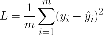

This function, as the name implies, is the average squared difference between the model output, yhat, and the actual value, y. The sum is taken over all m data points. If you use a different set of parameters, you will get a different set of predictions, and therefore a different loss.
If we can find the model parameters that minimize this value, we may have a good model!
Fitting the Model to Data
At this point, we have our linear model, and we have a function that tells us how well a given set of parameters is doing in terms of making accurate predictions on the dataset. We finally need to describe how you go about finding the best-fitting set of parameters. There are two main methods:
Analytically via the "Normal Equation"
Numerically via Gradient Descent (and similar approaches)
The first method, the analytical solution, provides us with exact best-fitting parameters in one step. As long as the problem is moderately small (~100s of input features or less), this is the way to go. With a dataset in hand, you can compute the best-fitting parameters via the following matrix transformations:

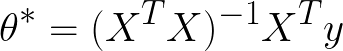
where X is the vector of input features, X = (x1, x2, x3...), and is the vector of labels y = (y1, y2, y3...). The benefit of being able to write down a simple solution for directly finding the best-fitting parameters is a feature of linear models.
The second method, gradient descent, can be used when the matrix inverse in the Normal Equation method is too slow. With gradient descent, you first compute the derivative of the cost function (in this case, the mean squared error) with respect to the model parameters. These derivatives tell us, for a given value of the model parameters, whether we should increase or decrease each model parameter to minimize the loss. For the MSE, the derivatives are given below:

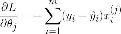
You will have as many derivatives as you do features. The superscript (j) indicates the jth feature/parameter, while the subscript (i) indicates the ith data point. Therefore, to compute the derivative of the loss with respect to theta1, you sum the differences between the data and the model (y_i - yhat_i), multiplying each term by the jth feature of the ith data point.
We start with an initial guess of the model parameters, which can be set arbitrarily. Then we compute the derivatives, plugging in the current value of our model parameters. Finally, we adjust our parameters iteratively:
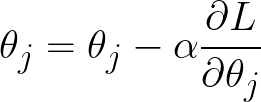

Alpha is known as the learning rate and is a common feature of many machine learning algorithms. It controls the magnitude of the parameter update at each step. If the steps are too large, you may overshoot the minimum and fail to converge. If the steps are too small, it may take forever to converge. In practice, you will have to adjust this parameter to get a sense of what learning rate works best for your problem.
Thanks for reading my very first article! Stay tuned for Part 2 in the Machine Learning Fundamentals series, where we will fit a linear model to data using Python!