In my last machine learning article, I explained the basics of linear regression. Today, we're going to write our own linear regression routine from scratch.

Let's dive in!

Some Mathematical Preliminaries

Last time, we introduced the linear hypothesis function:

I would like to make a small modification to the function to give our model just a bit more flexibility. It is conventional to add a constant term, also known as a bias:

You can think of this model as having an extra null feature, x0, that is always equal to 1:

This allows us to express the sum as a dot product for compactness:

We can use numpy's dot product for fast, parallelized computation.

import numpy as np

Coding a Linear Regression Model in Python

In the last article, I explained that there were two ways to solve for the best-fitting parameters on a given dataset. The first method was using the normal equation:

We can solve this equation for a given dataset using numpy's built-in linear algebra functions.

def normal(X, y):
        # best fitting thetas = [Xt*X]^-1*Xt*y
        Xt = np.transpose(X)
        inverse_xtx = np.linalg.pinv(np.dot(Xt, X))
        return np.dot(np.dot(inverse_xtx, Xt), y)

This method gives us the set of parameters that minimizes the mean squared error. The normal equation not only gives us exact answers, but can be expressed in concise code. The drawback is the cost of computation when the number of features grows large.

The second method for fitting the model is gradient descent, which iteratively improves the model by adjusting the parameters in such a way to decrease the mean squared error. This will require a few functions. First, let's write a function to express our hypothesis function:

def h(X, theta):
    return np.dot(X, theta)

Now we'll write a function that will represent a single step of gradient descent. This function will be called over and over as we update our parameters.

 def gradient_descent(X, y, theta):
        m = len(X) # Number of training examples
        error = y - h(X)
        dthetas = -np.dot(error, X)/m
        loss += sum((error**2)/m)
        return (dthetas, loss)

Following the equation for the derivative of the loss function as we discussed in the previous article, we first compute the error for each training example, y - h(X). Then, we compute the dot product between this error and the jth feature. We can sum up the individual errors on each data point to compute the total loss. Both the loss and the derivatives with respect to each parameter are returned.

The last thing we need for gradient descent to work is to iterate through the data over and over, updating the parameters at each state. One iteration through the data is known as an epoch:

for epoch in range(0, epochs):
    dthetas, loss = sgd(X, y)
    sys.stdout.write("\rEpoch: {}, Loss: {}, Thetas: {}".format(epoch, loss, theta))
    sys.stdout.flush()
    theta += alpha*dthetas

Creating A Sample Dataset

I wrote a small function to produce a sample dataset. It generates a 50 points on a line with a slope = pi (3.14159...), and y-intercept = 0, and adds normally distributed noise (mean = 0, std = 0.5).

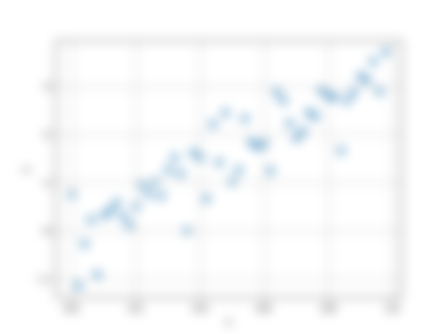
All real datasets have noise, which can arise due to a number of factors, including measurement error or sampling biases. Regardless of the source, noise hinders our ability to learn. The goal of all machine learning models is to extract the meaningful signal from the noise.

Now that we have a dataset, we're ready to fit our model!

Fitting the Model

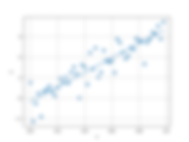
First we can fit the model to the data using the Normal Equation - here is the result:

theta0 = -0.16656555  
theta1 = 3.54015443

Recall that the underlying line that the data was generated from corresponds to theta0 = 0, theta1 = pi. Given the large amount of noise in the dataset, the algorithm learned the parameters reasonably well:

Next, we try the gradient descent method. We have two hyperparameters we can tune: alpha (learning rate) and the number of epochs. Using alpha = 0.01, and epochs = 10000, the algorithm will converge to roughly the same parameters:

Epoch: 10000, Loss: 0.23948526551145863
theta0 = -0.16484926
theta1 = 3.53688388

You may have to use some trial and error to find the set of hyperparameters that give the most efficient learning. Keep in mind that depending on the complexity of the problem, you may not have time for a full exploration of the space of hyperparameters.

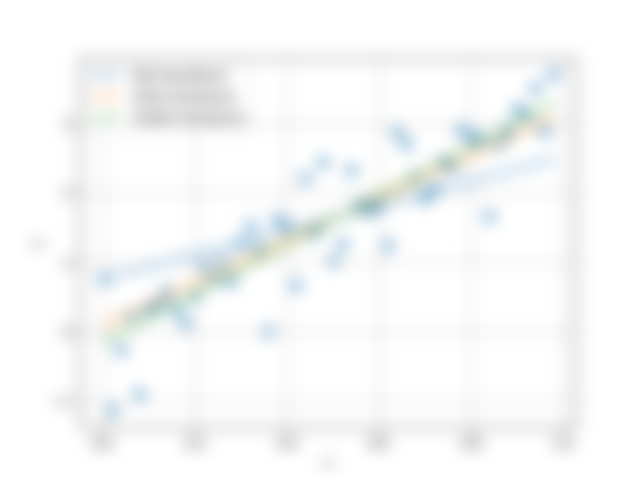
For a final check, I plotted the models fitted with 500, 2500, and 10,000 gradient descent iterations to see how it converges:

Thanks for reading! Stay tuned for more articles on statistical modeling and machine learning.